Examples¶

MT: COMMEMI 3D-2¶

We use COMMEMI 3D-2 model (Fig. 1) to verify the correctness of the developed method by comparing our results with those produced by ModEM. For this problem, we refined the mesh locally around the receiver points and the two central blocks. The resulting mesh has 2.1 million cells and 2.5 million edges (Fig. 2). Fig. 3 compares the numerical solution along y=0km with ModEM.

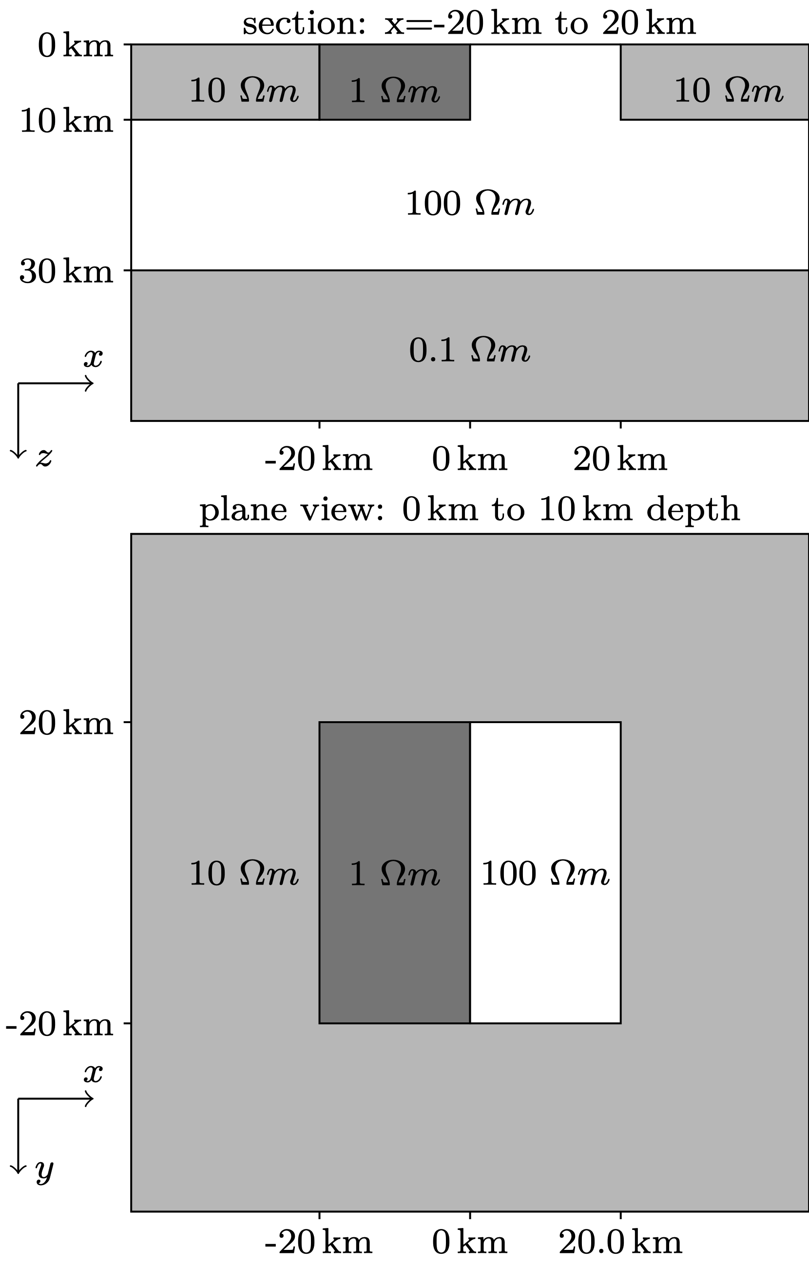
_images/commemi3d2-mdl.png — Fig. 1 Sketch of COMMEMI 3D-2 model¶

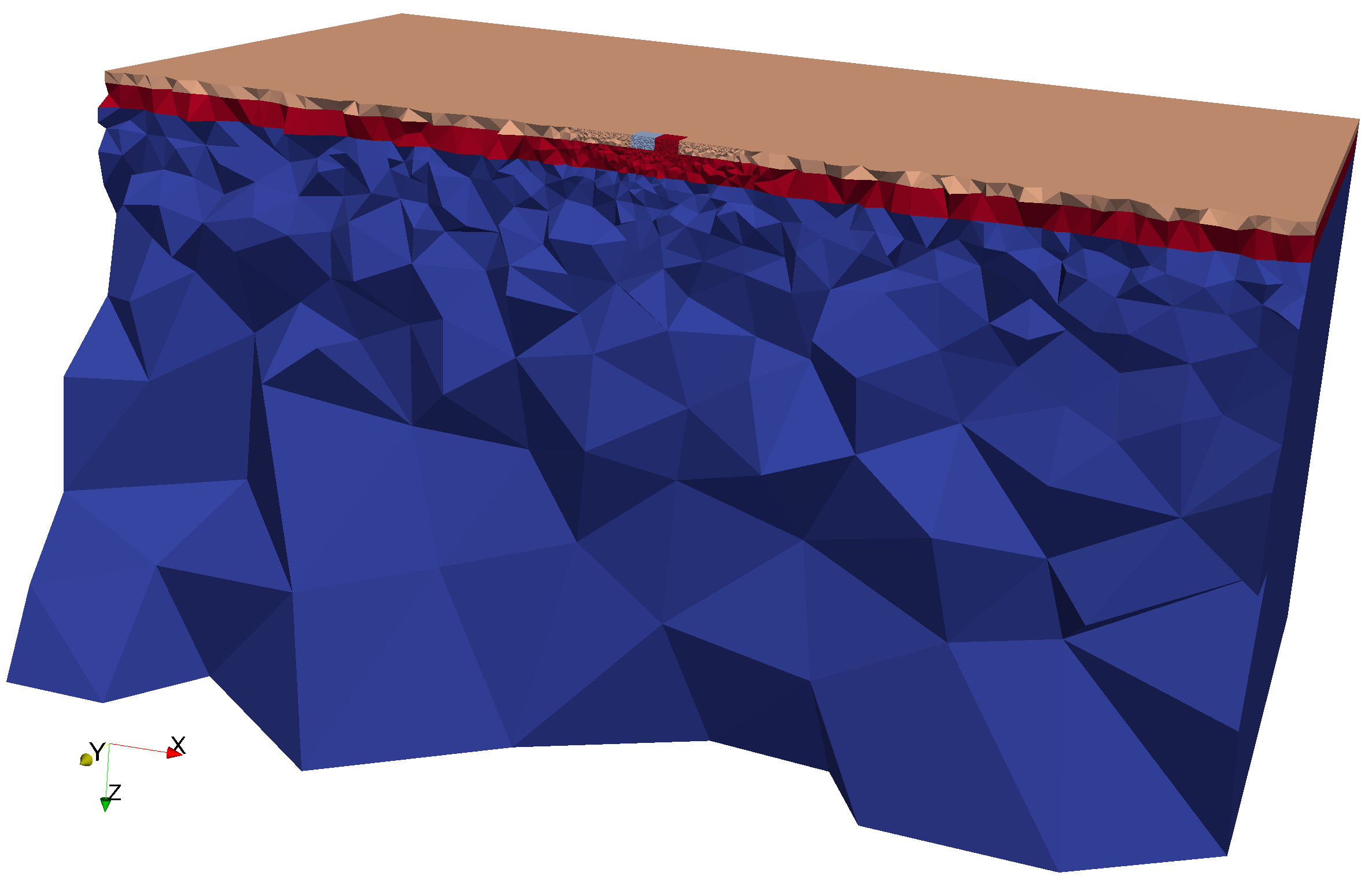
_images/commemi3d2-mesh.png — Fig. 2 Locally refined mesh used to generate the response¶

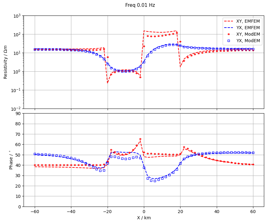
_images/commemi3d2-0.01Hz.png — Fig. 3 Apparent resistivities and phases calculated for COMMEMI 3D-2 model at a frequency of 0.01 Hz¶

MCSEM: 3D Reservoir Model¶

The following is a marine CSEM example. The model contains a reservoir block of resistivity 100 \(\Omega m\) located 1km under the seafloor. The geometry of the reservoir is \(2km \times 3km \times 0.1km\). A \(y\)-directed electrical dipole was placed at \((0km, -4km, 0.9km)\). 121 receivers were place at the seafloor for -6km to 6km along the y direction.

The computational domain was discreted into tetrahedron elements. Fig. 4 shows the initial mesh. Fig. 5 show the final mesh after 5 adaptive mesh refinements.

We also computed the response of the model, as well as the response of the background model (without reservoir block) and compared with Kerry Key’s Dipole1D, as shown in Fig. 6.

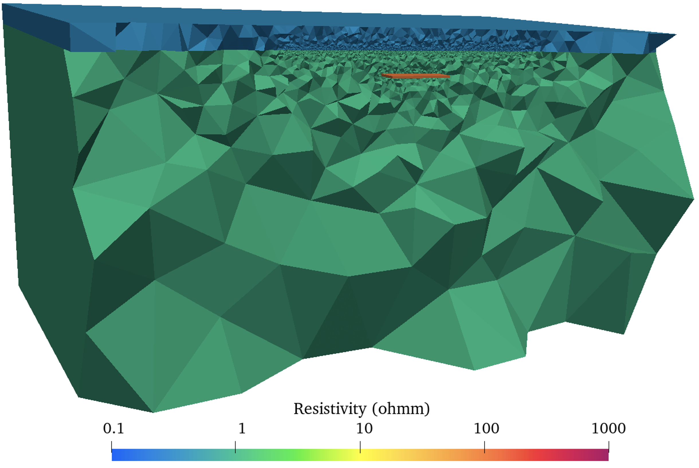
_images/mcsem-initial-mesh.png — Fig. 4 Initial mesh of the marine CSEM reservoir model.¶

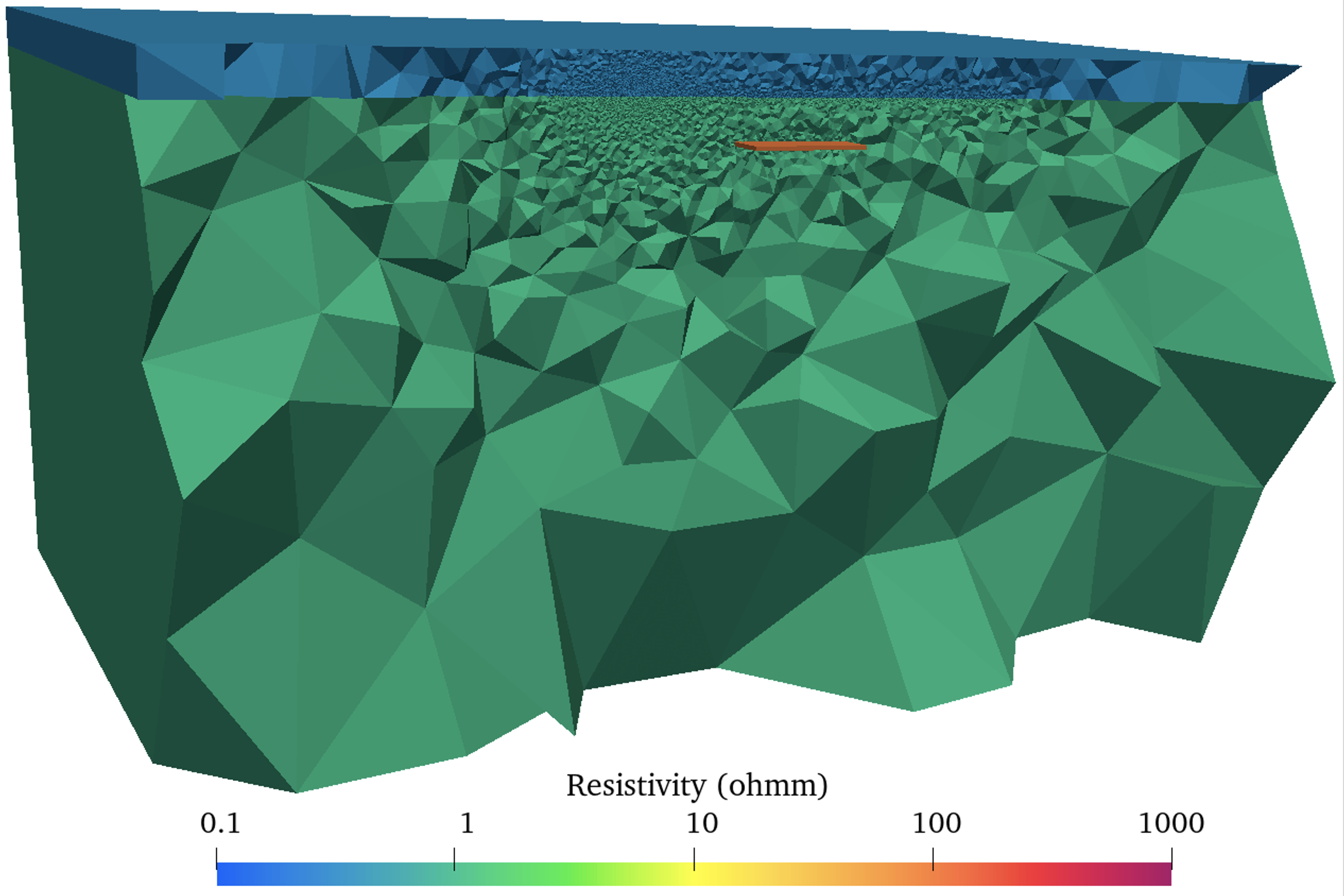
_images/mcsem-final-mesh.png — Fig. 5 Final mesh of the marine CSEM reservoir model after 5 adaptive mesh refinements¶

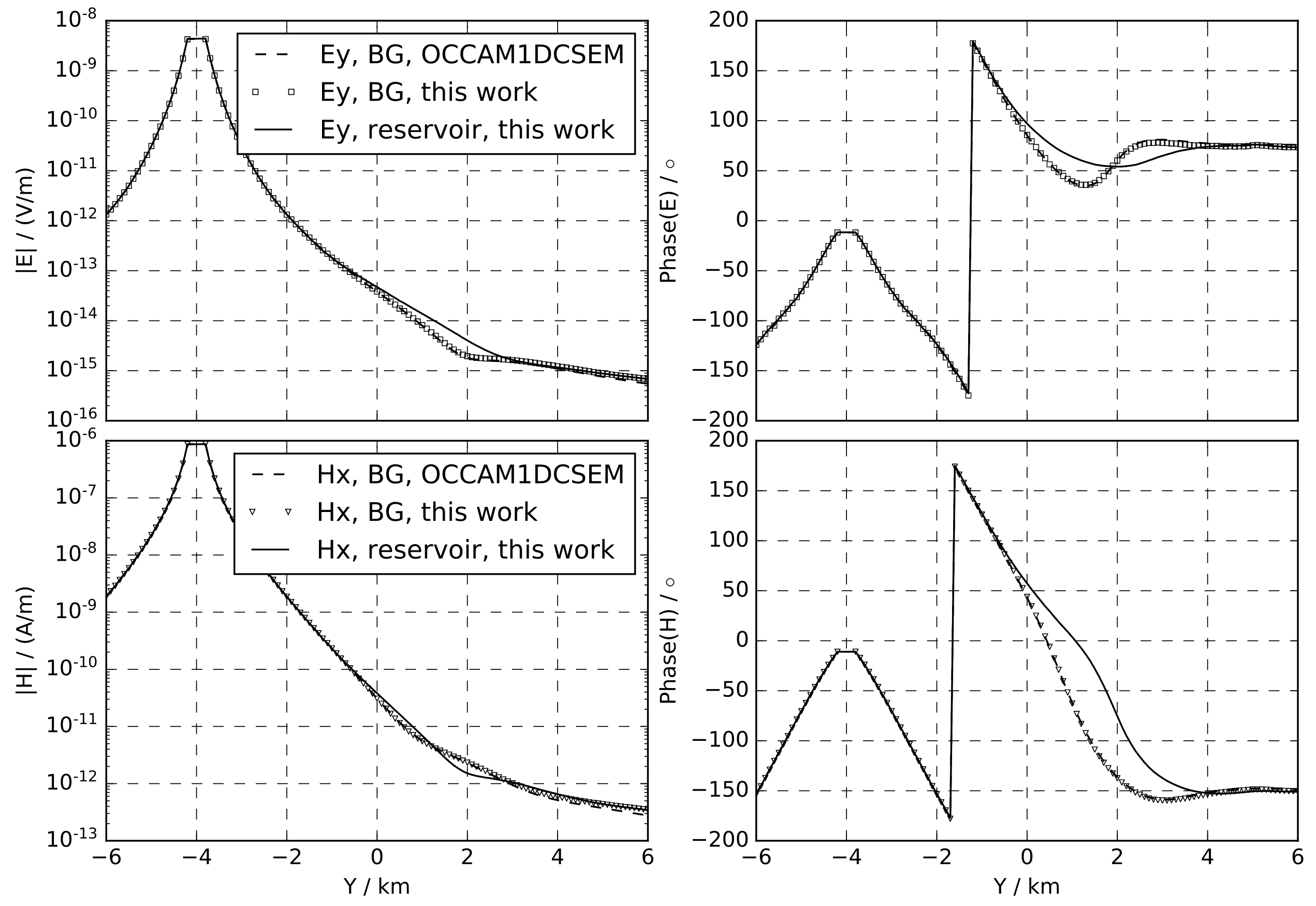
_images/mcsem-response.png — Fig. 6 Response of the reservoir model.¶

MT anisotropic model¶

EMFEM supports general anisotropic media. Here is an example. This model was designed by Yuguo Li (Yuguo Li, 2002, GJI). It contains a 2D slab anisotropy in a half-space of 1000 \(\Omega m\). The conductivity tensor of the slab is given by the principal resistivities 500/10/500 \(\Omega m\) for varying dip angles \(\beta\), as shown in Fig. 7. Fig. 8 and Fig. 9 show the apparent resistivities of the model for various dip angles \(\beta=0/30/60/90\).

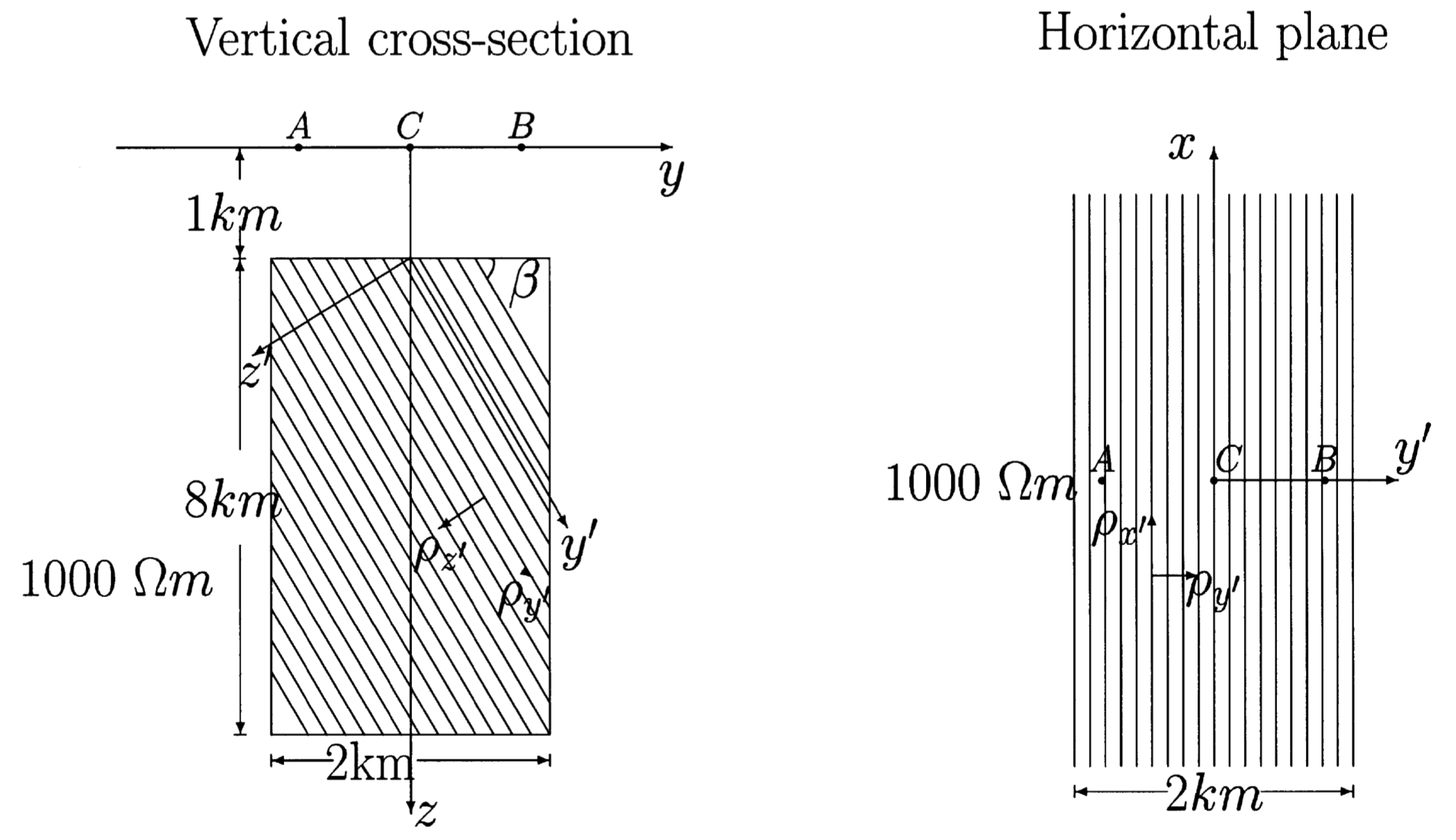
_images/li2002-mdl.png — Fig. 7 A 2D slab anisotropy model. Figure courtesy of Yuguo Li.¶

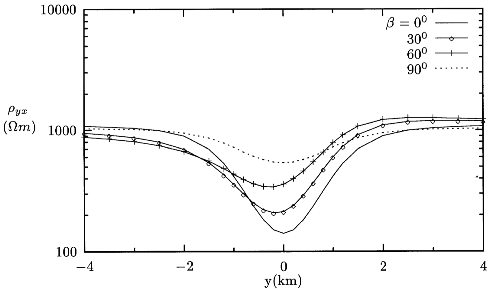
_images/li2002-rsp-li.png — Fig. 8 Apparent resistivities at a frequency of 0.1 Hz, shown in (Li, 2002, GJI). Figure courtesy of Yuguo Li.¶

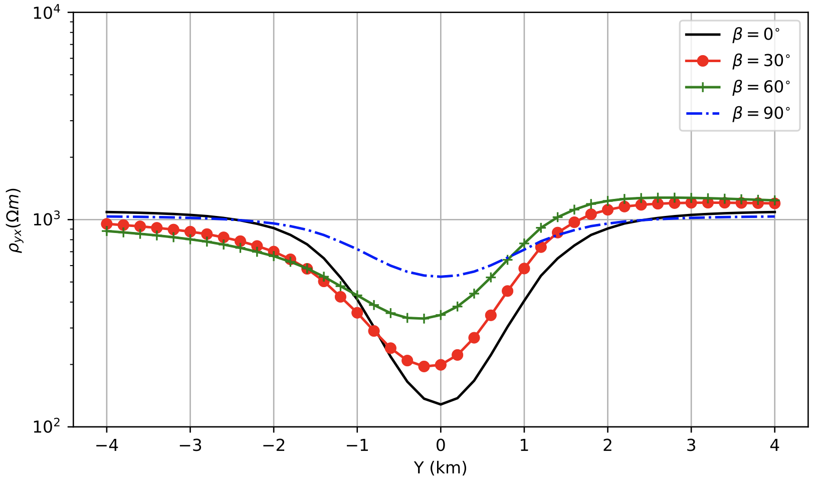
_images/li2002-rsp-emfem.png — Fig. 9 Apparent resistivities calculated by EMFEM.¶